Plotting spatial residuals

2022-06-17

Here we will use the vista package to display spatial residuals from spatiotemporal models

library(vista)
library(mgcv)
data(pcod)

GAM with spatial smooths by year

We’ll use a GAM for demonstration purposes, but any other package randomForest, sdmTMB, etc. could be used instead.

m <- gam(density ~ 0 + as.factor(year) + s(X,Y,by=as.factor(year)), 
         data=pcod, family=tw())
pcod$pred = predict(m)
pcod$resid = residuals(m)

Predictions in space

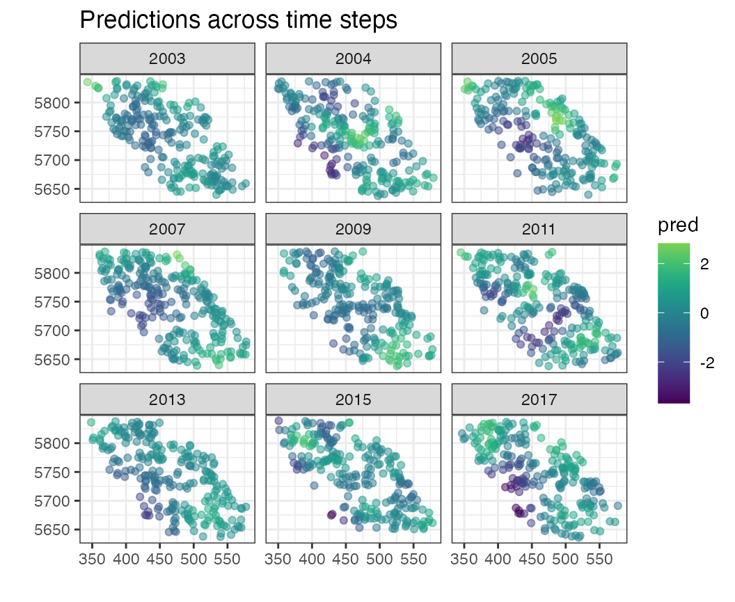
The pred_space function plots predictions spatially. By default, removes temporal means so the predictions in each time slice have mean 0. By default, the predictions are faceted by time,

pred_space(df = pcod, time = "year")

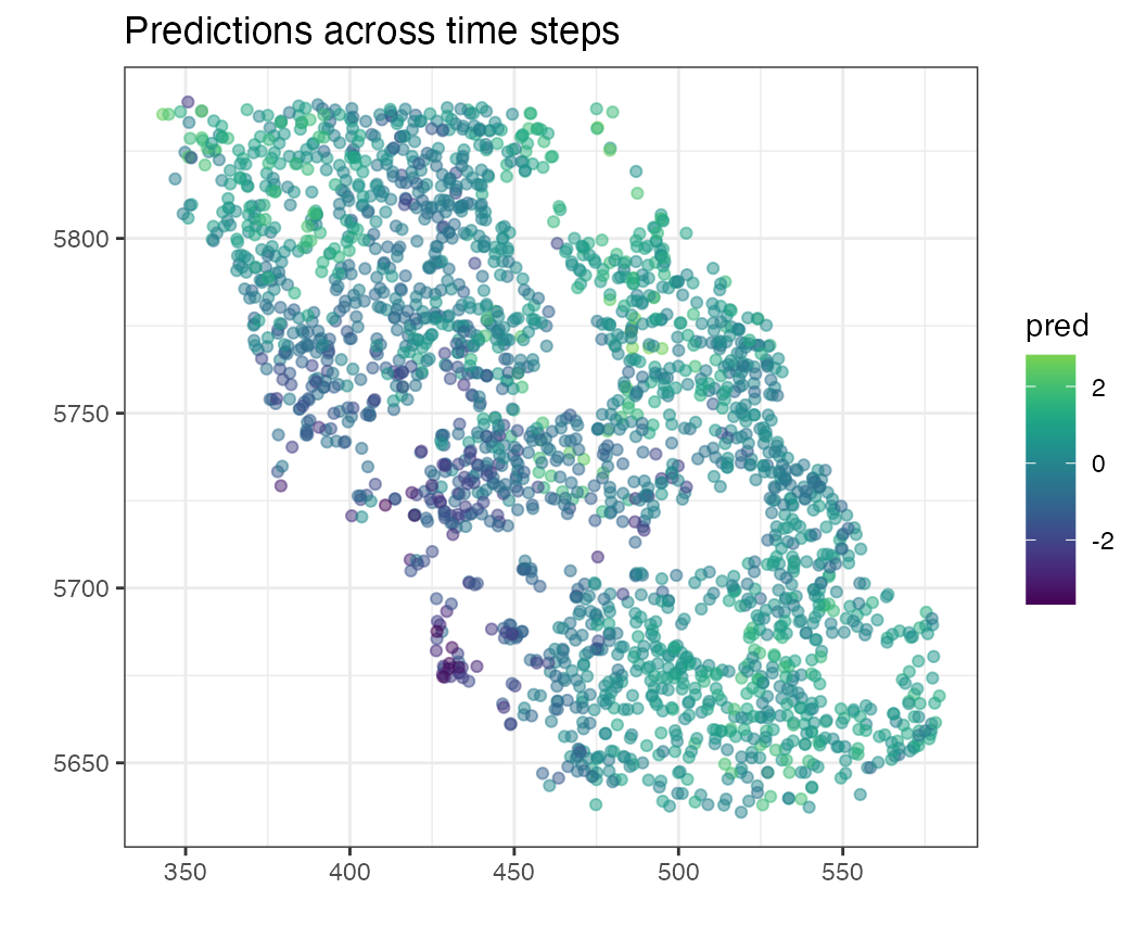
But we can also turn off faceting using by_time

pred_space(df = pcod, time = "year", by_time = FALSE)

Residuals in space

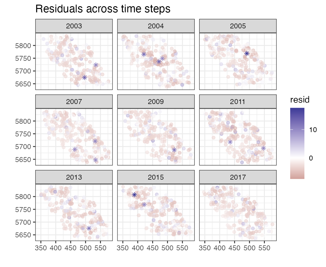
Similarly, the resid_space function is designed to plot spatial residuals (again these have mean 0). And faceting can be turned on / off, but by default by_time = TRUE.

resid_space(df = pcod, time = "year")

QQ plot spatially

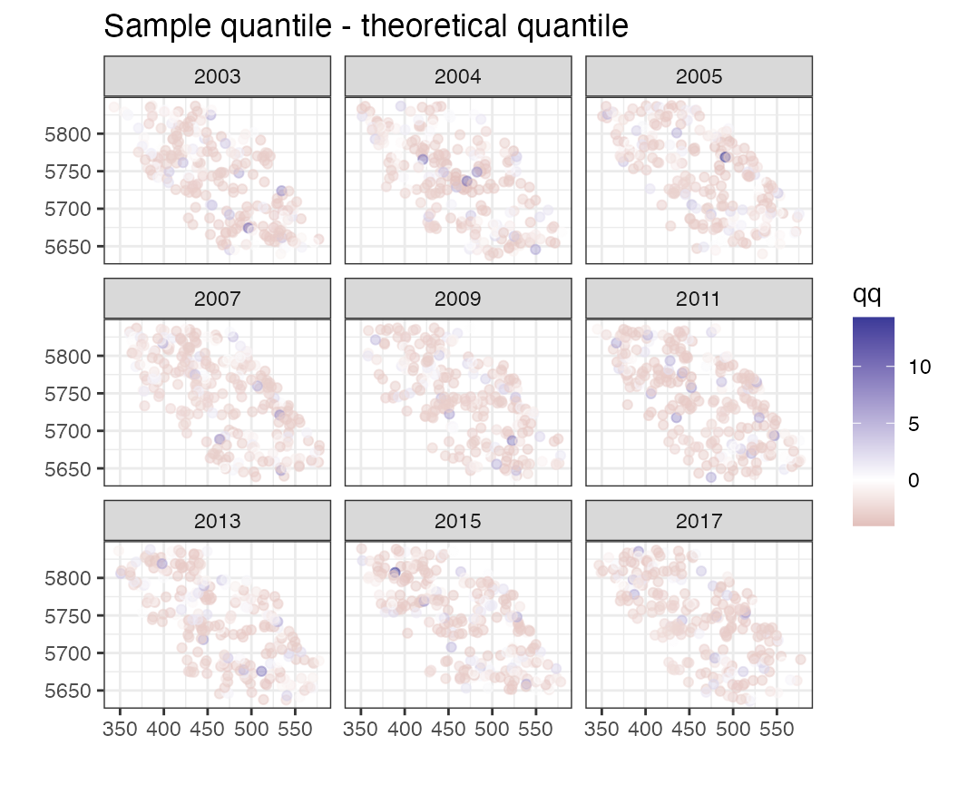
The qq_space function is also useful in displaying the quantile residuals (via a call to stats::qqnorm)

qq_space(pcod, time = "year")