Plotting temporal residuals

Here we will use the vista package to plot temporal residuals from spatiotemporal models

library(vista)
library(mgcv)
data(pcod)

GAM with spatial smooths by year

We’ll use a GAM for demonstration purposes, but any other package randomForest, sdmTMB, etc. could be used instead.

m <- gam(density ~ 0 + as.factor(year) + s(X,Y,by=as.factor(year)), 
         data=pcod, family=tw())
pcod$pred = predict(m)
pcod$resid = residuals(m)

Predictions through time

The pred_time function displays the range of predictions across time slices.

pred_time(df = pcod, time = "year")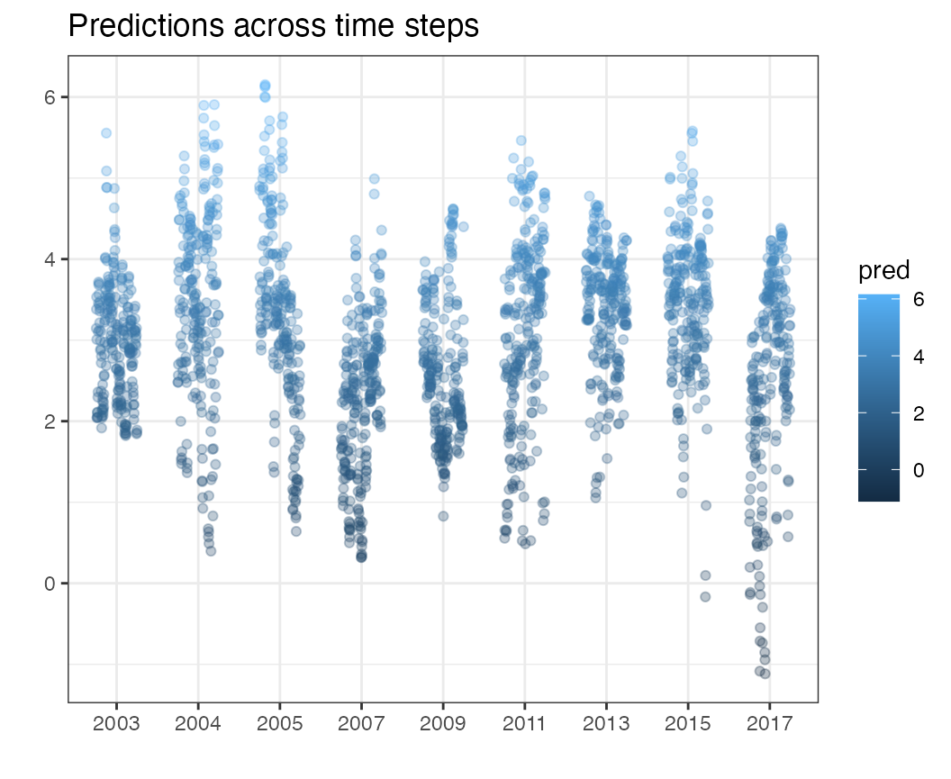

Residuals through time

Similarly, the resid_time function is designed to plot residuals across time slices

resid_time(df = pcod, time = "year")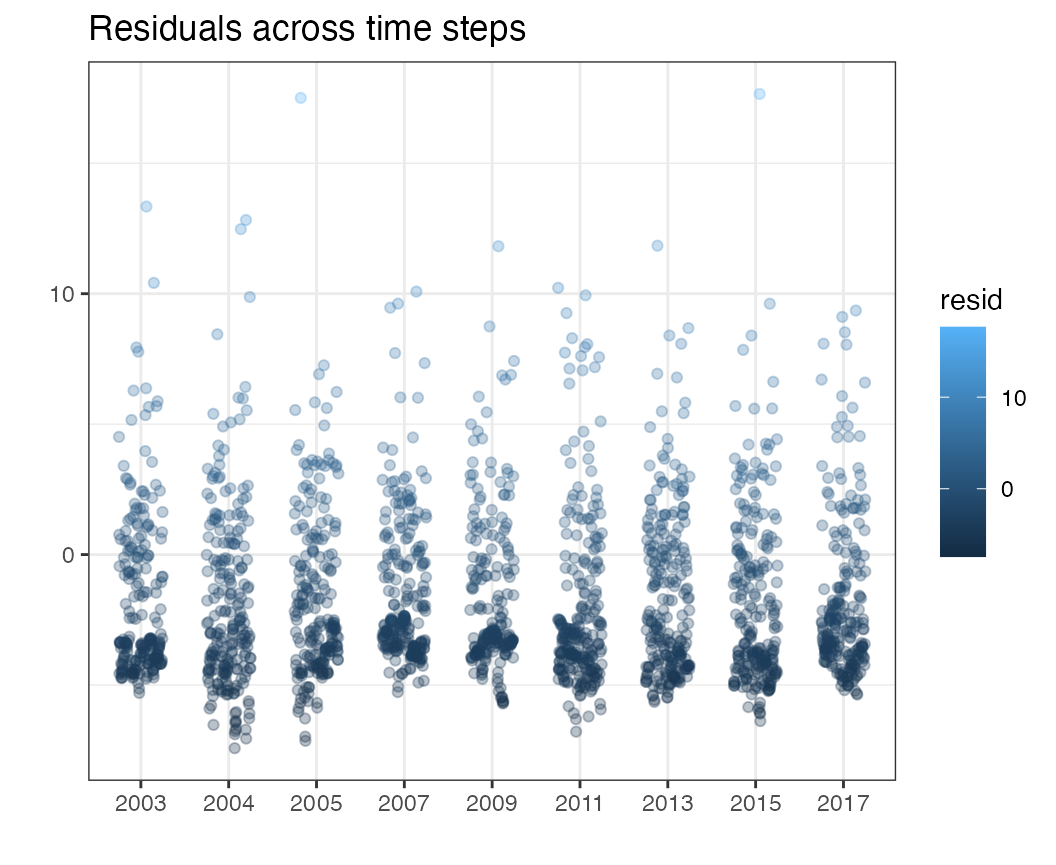

Homogeneity of residuals through time

In some cases, the variability of a spatial process may be non-stationary and increasing or decreasing over time. We can visualize this using the sd_resid_time function, where ideally there is no trend or outlier.

sd_resid_time(df = pcod, time = "year")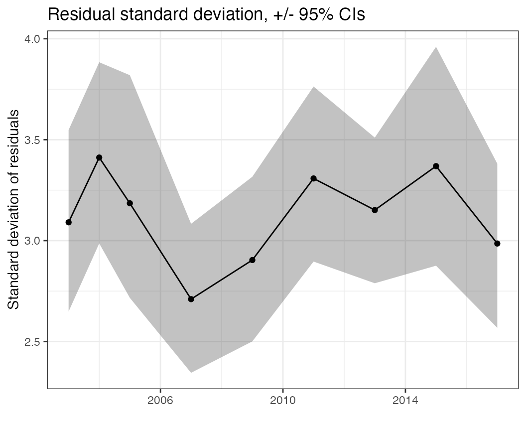

QQ plot temporally

The qq function is also useful in displaying the quantile residuals (via a call to stats::qqnorm). By default this will be faceted by time, but faceting can be turned off with by_time = FALSE.

qq(pcod, time = "year")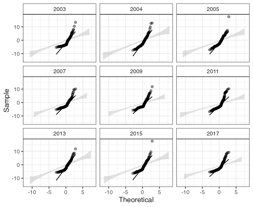

Scale - location plots

The scale_loc function displays scale - location plots, which may be useful at diagnosing trends in residuals vs predicted values,

scale_loc(df = pcod, time="year")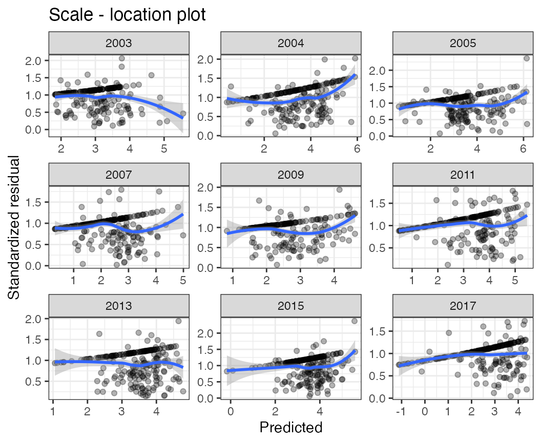

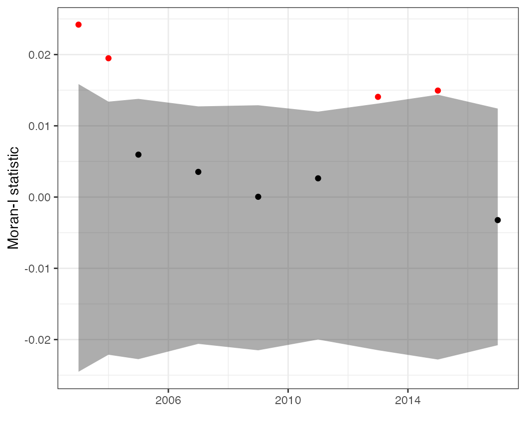
Moran’s I statistics

We can calculate lots of variants of Moran’s I. The moran_ts plot is useful for displaying time series of the Moran-I statistic, calculated separately for each time slice. This can be done on predicted values,

moran_ts(df = pcod, time = "year", response = "pred")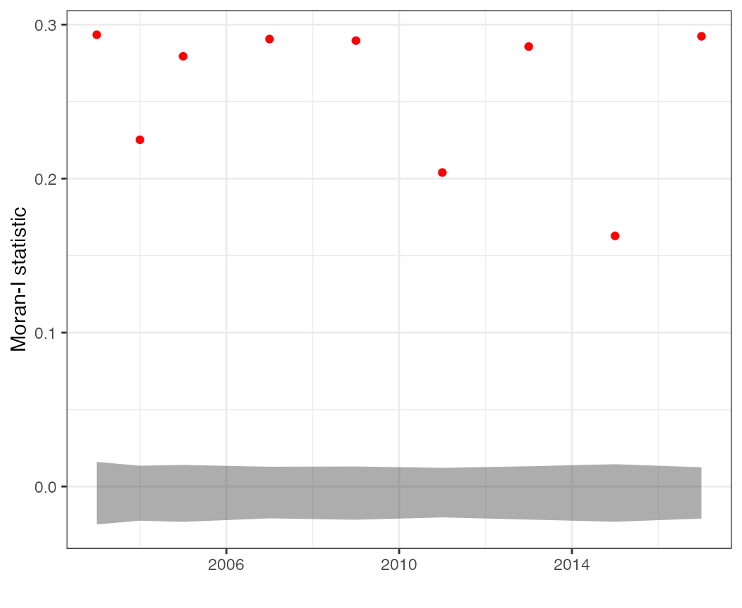

But if a goal is evaluating whether a particular model removes spatial autocorrelation, it may be more useful to calculate this on the residuals,

moran_ts(df = pcod, time = "year", response = "resid")