Overview of the vista package

Here we will use the vista package visualize output from spatiotemporal models

library(vista)

Data

Each of the functions in the vista package takes a generic data frame as an argument. As some examples, we can fit models to the pcod example dataset from Pacific cod in the sdmTMB package, collected by Fisheries and Oceans Canada.

1. sdmTMB

sdmTMB is a package for fitting generalized linear mixed models (GLMMs) with spatial and spatiotemporal Gaussian random fields. The package can be installed here,

remotes::install_github("pbs-assess/sdmTMB")
library(sdmTMB)

data(pcod)

We fit a fairly simple spatiotemporal model, using an example from the package. Don’t worry about all the arguments – the density of Pacific cod is modeled as a function of fixed effects (years) and spatiotemporal random fields (essentially different spatial maps in each year). The response is modeled with a Tweedie distribution.

mesh <- make_mesh(pcod, c("X", "Y"), cutoff = 15)
m <- sdmTMB(
  data = pcod,
  formula = density ~ 0 + as.factor(year),
  time = "year",
  mesh = mesh,
  family = tweedie(link = "log"),
  spatial = "off"
)

Next, we can calculate the residual and predicted values from the fitted model

pcod$pred <- predict(m)$est
pcod$resid <- residuals(m)

2. generalized additive models (GAMs) in mgcv

library(mgcv)
m <- gam(density ~ 0 + as.factor(year) + s(X, Y, by = as.factor(year)),
  data = pcod, family = tw()
)

Again, calculate the residual and predicted values

pcod$pred <- predict(m)
pcod$resid <- residuals(m)

3. random forest models

library(randomForest)
m <- randomForest(density ~ year + X + Y + X:Y, data = pcod)

Objects of class randomForest can be used with the predict function, but because these are non-parametric methods, some of the plots in the vista package (specifically those focused on residuals) won’t work.

pcod$pred <- predict(m)

Types of plots

We can use the vista package to generate diagnostic plots. Each plot can be run individually. Some example functions are below (illustrating how to use them with our pcod example above):

# Look at all predictions over space, faceted by time (or not)
pred_space(df = pcod, time = "year")
# Look at all predictions time
pred_time(df = pcod, time = "year")
# Look at residuals over space, faceted by time (or not)
resid_space(df = pcod, time = "year")
# Look at all residuals over time
resid_time(df = pcod, time = "year")
# Look at variation in residuals through time
sd_resid_time(df = pcod, time = "year")
# Look at variation in residuals across space, faceted by time (or not)
sd_resid_space(df = pcod, time = "year")
# Look at qq plots, faceted by time (or not)
qq(df = pcod, time = "year")
# Look at qq plots over space, faceted by time (or not)
qq_space(df = pcod, time = "year")
# Look at predictions vs residuals, faceted by time (or not)
pred_resid(df = pcod, time = "year")
# Look at time series of Moran statistics (e.g. residuals, predicted values)
moran_ts(df = pcod, time = "year")

Examples

As an alternative to generating plots individually with specific functions, we can call the wrapper function to run all plots. This is a lot more convenient, and returns a list of ggplot() objects.

plots <- diagnostic_plots(pcod, time = "year")

We can inspect the plots individually, e.g.

names(plots)

##  [1] "pred_space"         "pred_space_bytime"  "pred_time"         
##  [4] "resid_space"        "resid_space_bytime" "resid_time"        
##  [7] "sd_resid_time"      "sd_resid_space"     "qq"                
## [10] "qq_time"            "qq_space"           "pred_resid"        
## [13] "moran_pred"         "moran_resid"        "scale_loc"         
## [16] "scale_loc_time"

Or look at them individually. For example we can look at the residuals spatially, and across time slices with

plots$resid_space_bytime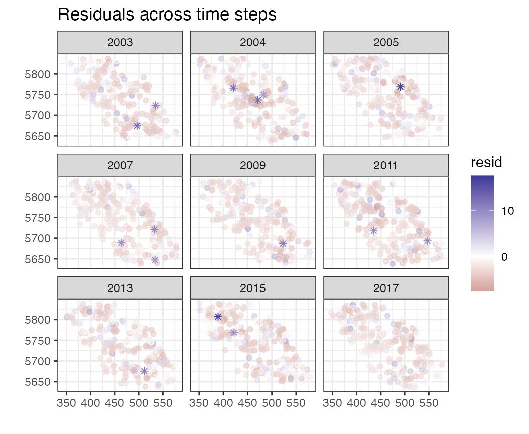

This may not be informative (because residuals are often on different scales). Instead we can look at the randomized quantile residuals,

plots$qq_space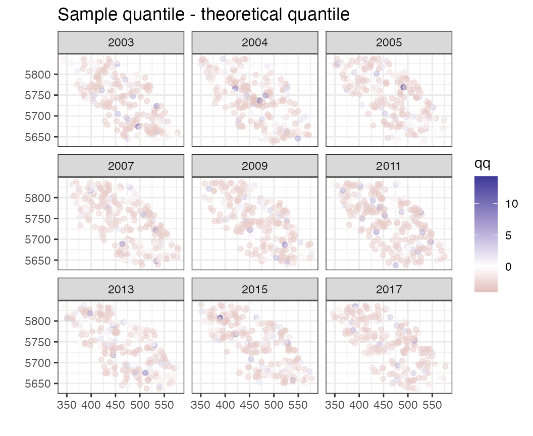

Some plots are specific to particular models. For example, looking at the mean residuals over space, all values are 0 because each row of the dataframe has a unique (X,Y) coordinate – as opposed to repeat sampling at fixed stations.

The standard deviation of residuals over time seems to maybe suggest higher variability earlier in the time series, but not a trend in the variation over time

plots$sd_resid_time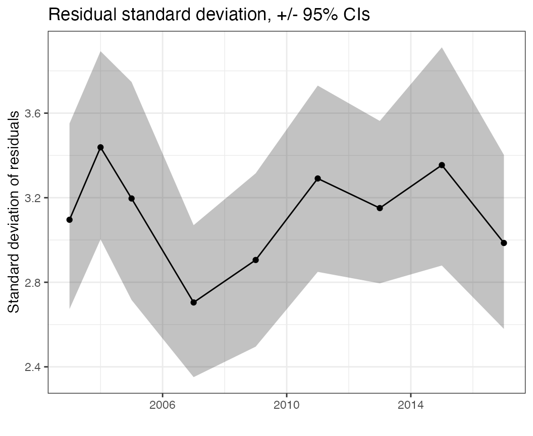

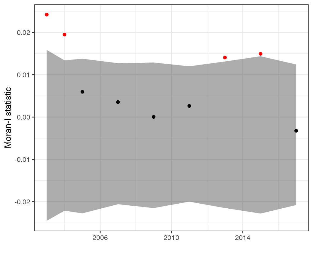
Additional statistics (such as the Moran statistic) can be used to diagnose lingering spatial autocorrelation. These plots can be made on the predictions (where we expect there to be spatial autocorrelation)

plots$moran_pred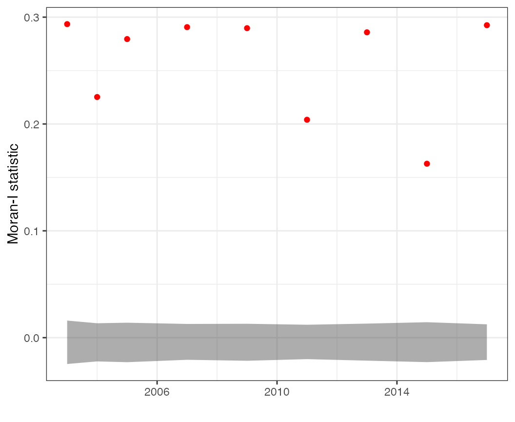

or on the residuals, where we hope there is little residual autocorrelation (because our spatial model is explaining away most of it).